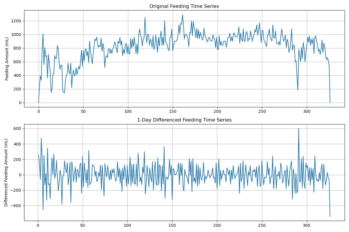
Forecasting Bottle Feeding with (S)ARIMA

After trying regression models on individual feeding events, I realized that predicting each point in isolation was noisy and unstable. Instead, I turned to binned data by aggregating bottle amounts into daily totals. This smoothed out random fluctuations and gave a clearer signal to model.

The basic tool I chose was Auto Regression Integrated Moving Average (ARIMA). Since the feeding data clearly has a long-term growth trend, I set the integration parameter I = 1. This tells the model to difference the series once, removing the overall drift so it can better capture short-term dynamics.

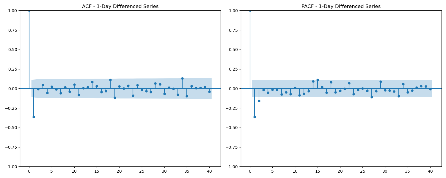
Daily totals — *Daily total bottle amounts, showing a smoother trend than individual feedings. Bottom) Amount with 1-Day differencing, showing noise-like pattern to remove long term trend.*

To decide how many coefficients to include, I used ACF (Autocorrelation Function) and PACF (Partial Autocorrelation Function) analysis. These plots reveal the “peaks” in the regression power spectrum, which guide the choice of autoregressive (AR) and moving average (MA) terms. Based on the diagnostics, I tested models up to second-order autoregression with a two-day moving average.

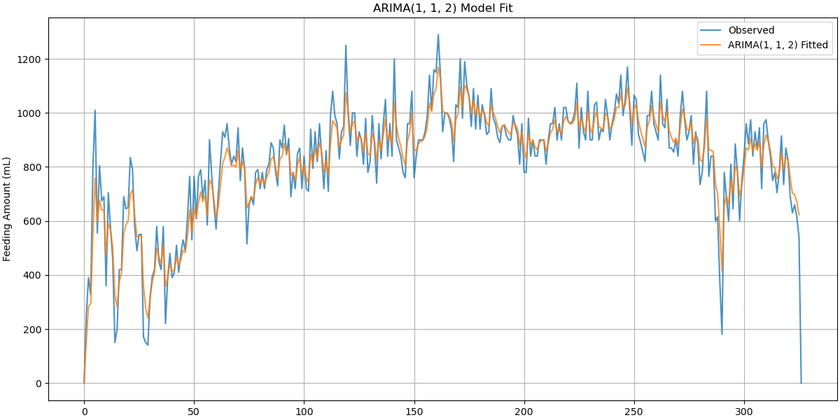
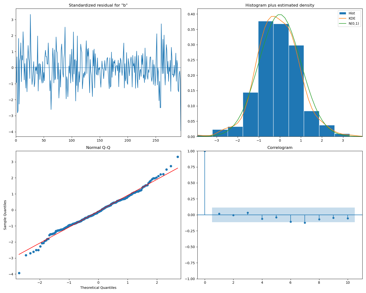
*ACF and PACF plots used to determine AR and MA order selection.*

I experimented with several configurations, including ARIMA(2,1,1) and related variations. Model performance was measured with Root Mean Squared Error (RMSE) and Mean Absolute Deviation (MAD). Most importantly, I inspected the residuals as another time series: a good ARIMA model should leave behind only random noise.

Arima Fit — *Fit and original data using the best ARIMA model.*

ARIMA Residuals — *Residual analysis: the best ARIMA model leaves residuals that resemble random noise.*

Next, I extended the analysis with SARIMA (Seasonal ARIMA). I tested seasonality of 7 days (weekly) and 30 days (monthly). However, neither performed well. The problem is that feeding patterns don’t follow simple calendar cycles. Instead, they show developmental growth spurts at irregular intervals: around 10 days, 3 weeks, 6 weeks, 3 months, 6 months, and beyond. These bursts aren’t well captured by fixed seasonal models.

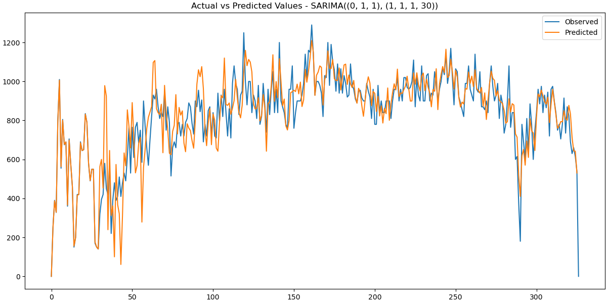
SARIMA Predictions — *SARIMA predictions compared with actuals. Seasonal terms struggled with rapid growth spurts.*

SARIMA Diagnostics — *SARIMA residual diagnostics.*

I could keep trying several version of the model orders. To automate the search, I tried autoARIMA, which scans through parameter combinations and returns the best model by information criteria. The results often converged on odd specifications like ARIMA(1,1,1)(1,1,1) or ARIMA(1,1,1)(1,1,0) (where are the second order parameters I expected?), which hinted that the data didn’t match clean seasonal cycles.

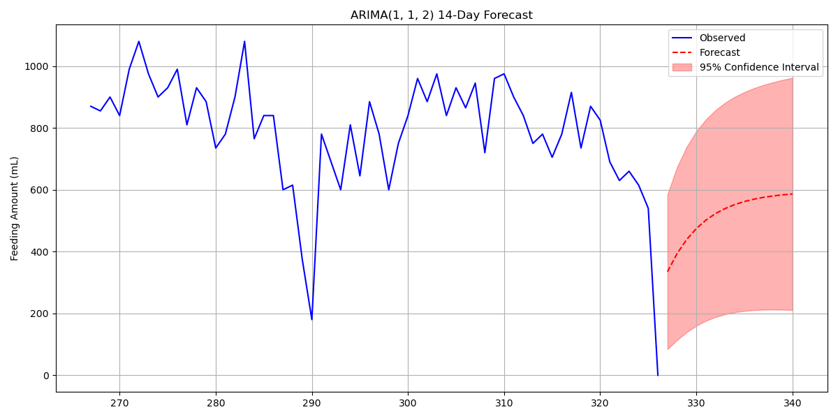
In the end, I stuck with the most stable model and generated 14-day forecasts. The predictions worked well for the earlier parts of the dataset but deteriorated in recent periods. This may be due to small sample sizes or noisy data, or from occasional logging mistakes or “weird days” where the baby deviated from routine.

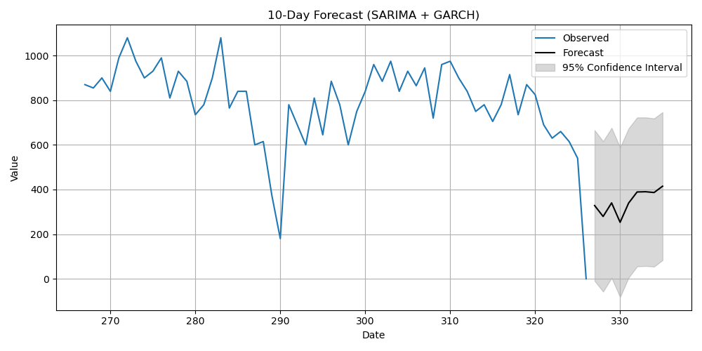
ARIMA 14-Day Forecast — *Forecast of bottle amounts over the next 14 days. Early predictions fit well, while later points diverge. This forecast grows, while in the previous regression model it decreased.*

SARIMA 14-Day Forecast — *Forecast of bottle amounts over the next 14 days. Early predictions fit well, while later points diverge. This forecast grows, while in the previous regression model it decreased.*

A likely next step is to combine strategies. Feeding is both a time series problem and an event prediction problem. My plan is to explore survival analysis, where I form a framework that could merge (S)ARIMA forecasts of daily totals with survival predictions of the time to next bottle. Together, this blended approach might finally capture both the long-term rhythms and the short-term intervals that matter most in daily care.